IPython and Jupyter
IPython (Interactive Python) is a command shell for interactive computing in multiple programming languages, originally developed for the Python programming language, that offers introspection, rich media, shell syntax, tab completion, and history. In 2014, born out of the IPython Project was Project Jupyter, a non-profit, open-source project evolved to support interactive data science and scientific computing across all programming languages.
Time series
In mathematics, a time series is a series of data points indexed, listed, or graphed in time order. Most commonly, a time series is a sequence taken at successive equally spaced points in time. Time series analysis comprises methods for analyzing time series data to extract meaningful statistics and other characteristics of the data. Time series forecasting is the use of a model to predict future values based on previously observed values.
Importance of Time Series Analysis
Ample of time series data is being generated from a variety of fields. And hence the study time series analysis holds a lot of applications. Let us try to understand the importance of time series analysis in different areas.
-
Healthcare : An epidemiologist might be interested in knowing the number of people infected over the past years. Like in the current situation the researchers might be interested in knowing the people affected by the coronavirus over a period. Blood pressure traced over a period can be used in evaluating a drug.
-
Environmental Science : Environmental time series data can help us explain the rise in temperature over the past few years. Plot shows the temperature data over a period.
-
Economics and Finance : Budget studies, stock market fluctuations, etc.
Time Series Analysis is needed to predict the future based on past data values which are mostly dependent on time. It is used by researchers and executives to predict sales, price, policies, and production.
Benefits of Time Series Analysis
Time series analysis has various benefits for the data analyst. From cleaning data to understanding it — and helping to forecast future data points — this is all achieved through the application of various time series models, such as :
SARIMA
The Seasonal Autoregressive Integrated Moving Average (SARIMA) method models the next step in the sequence as a linear function of the differenced observations, errors, differenced seasonal observations, and seasonal errors at prior time steps. It combines the ARIMA model with the ability to perform the same autoregression, differencing, and moving average modeling at the seasonal level. The notation for the model involves specifying the order for the AR(p), I(d), and MA(q) models as parameters to an ARIMA function and AR(P), I(D), MA(Q) and m parameters at the seasonal level, e.g. SARIMA(p, d, q)(P, D, Q)m where “m” is the number of time steps in each season (the seasonal period). A SARIMA model can be used to develop AR, MA, ARMA and ARIMA models. The method is suitable for univariate time series with trend and/or seasonal components.
-
Trend : Increasing or decreasing pattern has been observed over a period. In this case, the gradually increasing underlying trend is observed. i.e., the count of passengers has increased over a period.
-
Seasonality : Refers to cyclic pattern. A similar pattern that repeats after a certain interval of time. In the airline passenger example, we can observe a cyclic pattern which has a certain high & a low point which is visible in all the interval.
The Given Problem
A dataset is given in which the number of COVID-19 cases is recorded daily for different regions of Germany over a period of one year; in essence, several time series - one for each region. The line notation of the data file is Region Id, Region Name, Date, Number of Cases, separated by a comma, and each line corresponding to a specific region and a specific date. Note that the number of cases is cumulative, i.e., the number given in the record for a date refers to the total number of cases up to that date. You are asked to apply time series analysis techniques (such as trend calculation, seasonality, etc.) to study the dataset, and construct a predictive model that predicts the number of cases for subsequent days by region. Also, evaluation of the accuracy of the predictive model, using metrics such as Mean Absolute Error (MAE) and Root Mean Square Error (RMSE), using part of the time series in question to construct the model, and evaluating on the part that has been kept hidden. For example, the first 11 months can be used for model construction and the last month can be used to evaluate the predictions. Finally, visualize the time series as well as the forecasts you will produce. (Bonus) You are asked the following question : is there any correlation between neighboring geographical areas based on the observed number of cases?
The Data we are using : Data
The libraries I am using
import pandas as pd
import numpy as np
import matplotlib.pyplot as plt
from statsmodels.tsa.seasonal import seasonal_decompose
from statsmodels.tsa.statespace.sarimax import SARIMAX
import itertools
from sklearn.metrics import mean_absolute_error as mae
from geopy.geocoders import Nominatim # For Bonus
from geopy.distance import geodesic # For Bonus
Tip: A quick way for disabling all warnings:
import warnings
warnings.filterwarnings("ignore")
warnings.simplefilter(action='ignore', category=FutureWarning)
Generating the Data Frames from the Data File
# Import data from data.txt.
big_data = np.loadtxt("https://www.nickdoulos.com/assets/data.txt", delimiter=',', skiprows=1,
                    dtype = [('IDs','U3'), ('Cities', 'U30'), ('Dates', 'U25'), ('Cases', 'i4')])
# Make a dataframe of the data.
big_df = pd.DataFrame(big_data)


# This function separates the data.txt to small parts.
def specific_rows_from_df(filePath, start, finish):
  rows = []
  for i in range(start, finish):
    rows.append(i)
  with open(filePath) as f:
    for i, line in enumerate(f):
        if i in rows:
          yield line


# This function separates the data.txt to all the different ID parts.
def generate_dfs(filePath, id):
  x = 0
  temp = 0
  counter = 0
  for lines in big_data:
    x += 1
  for i in range(x):
    if big_df['IDs'][i] == id:
      if temp == 0:
        temp = i
      counter += 1
  if id == 'DE2':
    gen = specific_rows_from_df(filePath, temp, counter + temp)
  else:
    gen = specific_rows_from_df(filePath, temp + 1, counter + temp + 1)
  data = np.loadtxt(gen, delimiter=",",
                  dtype = [('IDs','U3'), ('Cities', 'U30'), ('Dates', 'U25'), ('Cases', 'i4')])
  df = pd.DataFrame(data)
  return df
The first function we encounter is specific_rows_from_df() which is helpful for the next function which takes as an argument the data.txt file along with the initial and final rows I want to get from each file, and returns all the intermediate rows between the initial and final rows. The function in which you use this is generate_dfs() which again takes as an argument what data.txt file and the respective ID of the Data Frame I want to create in order to create a separate Data Frame for each ID. This function is essentially implemented via two variables where one stores the first ID location while the other counts how many times these IDs appear by passing these variables into specific_rows_from_df().
Generating the Daily Cases and Re-indexing the Data Frame
# This function calculates the Daily Cases and re-indexes the Data Frame with the Dates column.
def daily_cases_and_reindex(df):
  daily_cases = []
  for i in df.index :
    if i == 0:
      daily_cases.append(df['Cases'][i])
    else:
      daily_cases.append(df['Cases'][i] - df['Cases'][i-1])
  df['Daily Cases'] = daily_cases
  df['Dates'] = pd.to_datetime(df['Dates'])
  df = df.set_index('Dates')
  df = df.asfreq('D')
  return df
The function daily_cases_and_reindex() takes a Data Frame and returns it having created a new column of daily cases for the region based on the cumulative cases and having changed the index of the Data Frame based on the Dates column.
One example of how to create a Data Frame with a given ID (In this case ID = DE1) :
df1 = daily_cases_and_reindex(generate_dfs("www.nickdoulos.com/assets/data.txt", 'DE1'))
Analyzing and Applying SARIMA Model to a selected Data Frame
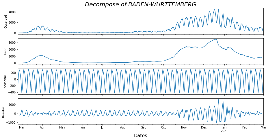
# Calculating and plotting the decomposed parts of df1 time siries.
def decompose(df_):
result = seasonal_decompose(df_['Daily Cases'], model='additive', extrapolate_trend=0)
plt.rcParams.update({'figure.figsize': (13,6.5)})
result.plot()
plt.xlabel('Dates', fontsize=16)
plt.title("Decompose of " + df_['Cities'][0], fontsize=20, pad='320.0', fontstyle='italic')
plt.show()
df_decomposed = pd.concat([result.seasonal, result.trend, result.resid, result.observed], axis=1)
df_decomposed.columns = ['Seasonality', 'Trend', 'Resid', 'Daily Cases']
# This function the optimal numbers for the SARIMA predictive model according to each AIC value.
def sarima_numbers_search(y,period):
p = q = d = range(2)
pdq = list(itertools.product(p, d, q))
seasonal_pdq = [(x[0], x[1], x[2],period) for x in list(itertools.product(p, d, q))]
mini = float('+inf')
for param in pdq:
for param_seasonal in seasonal_pdq:
try:
mod = SARIMAX(y, order = param, seasonal_order = param_seasonal,
enforce_stationarity = False, enforce_invertibility= False)
results = mod.fit()
if results.aic < mini:
mini = results.aic
param_mini = param
param_seasonal_mini = param_seasonal
except:
continue
print('The set of parameters with the minimum AIC is: SARIMA{}x{} - AIC:{}'
.format(param_mini, param_seasonal_mini, mini))
return param_mini, param_seasonal_mini
def forecast(df_):
# Creating a train and test set of the df_ dataframe for the predictive model.
df_ = df_.drop(['IDs', 'Cities', 'Cases'], axis=1)
to_train = df_[:'2021-01-31']
to_test = df_['2021-02-01':]
predict_date = len(to_test)
# Calculating the SARIMA predictive model.
my_param_mini, my_param_seasonal_mini = sarima_numbers_search(to_train, predict_date)
model = SARIMAX(to_train, order = my_param_mini, seasonal_order = my_param_seasonal_mini)
model_fit = model.fit(disp=False)
predicted = model_fit.forecast(predict_date)
predicted_df = pd.DataFrame(predicted, columns=['Predicted Daily Cases'])
# Calculating the Mean Absolute Error and the Root Mean Squared Error of the predicted values.
mse = ((predicted_df['Predicted Daily Cases'] - to_test['Daily Cases']) ** 2).mean()
mae_ = mae(to_test['Daily Cases'], predicted_df['Predicted Daily Cases'])
print('The Mean Absolute Error is : {}'.format(mae_))
print('The Root Mean Squared Error is : {}'.format(round(np.sqrt(mse), 2)))
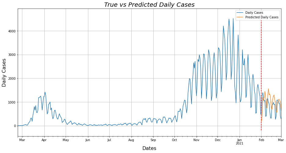
# Plotting the test and predicted values in the same figure.
ax = df_.plot()
ax.set_title('True vs Predicted Daily Cases', fontsize=20, fontstyle='italic')
ax.set_ylabel('Daily Cases', fontsize=16)
ax.set_xlabel('Dates', fontsize=16)
ax.vlines(['2021-02-01'], -200, 4700, linestyles='dashed', colors='red')
predicted_df.plot(ax=ax, figsize=(15.44, 7.70), logx=True, grid=True, alpha=0.95);
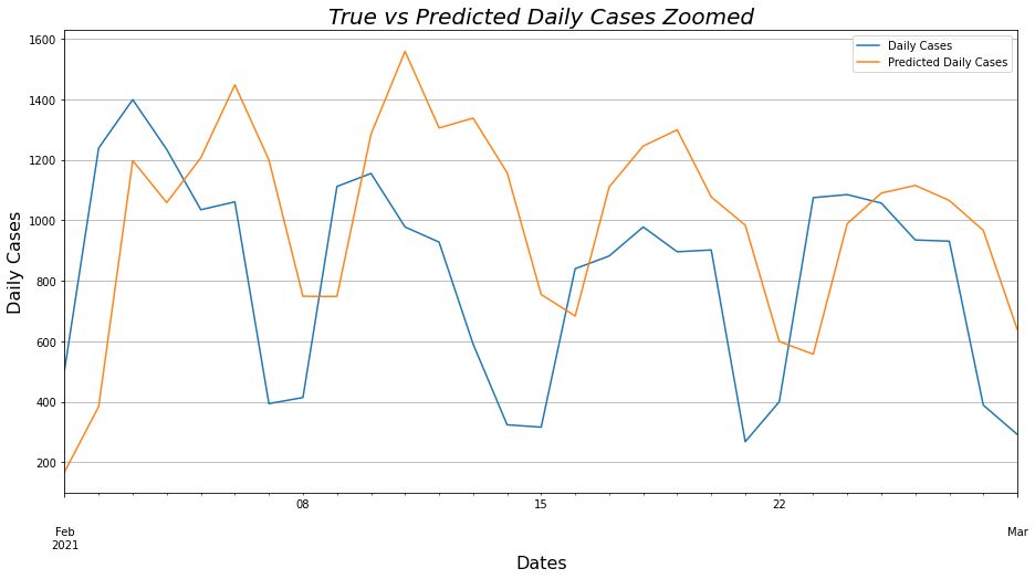
# Same plot just zoomed for more detail.
ax2 = to_test.plot()
ax2.set_title('True vs Predicted Daily Cases Zoomed', fontsize=20, fontstyle='italic')
ax2.set_ylabel('Daily Cases', fontsize=16)
ax2.set_xlabel('Dates', fontsize=16)
predicted_df.plot(ax=ax2, figsize=(15.44, 7.70), logx=True, grid=True, alpha=0.95);
decompose(df1)
forecast(df1)
Lets start analyzing the decompose() from the beginning. First we compute all the different pieces that make up a time series by means of the seasonal_decompose() function, which returns the seasonality, trend, time series residual and the time series itself and then these values are being plotted. Followingly, we remove from the Data Frame the columns that do not have any useful information and create two smaller Data Frames, one containing the first 11 months of Daily Cases to be used in the predictive model and another which will be the last month and this will be used to compare how close to reality the prediction is. The function sarima_numbers_search() increases the program execution by 2.1 minutes and computes the 6 variables which are necessary for optimal prediction, as all possible combinations of these 6 variables are calculated and the set of variables which have the smallest AIC - (Akaike Information Criterion) is selected which is a number by which the prediction models are compared with each other and the smaller this number is the “better” the prediction is most of the time. Finally, we run the SARIMAX Predictive Model via the forecast() function with the 6 variables taken from the previous function and the number of days we want to predict and create a new Data Frame with the predicted values. Then we calculate the MAE - (Mean Absolute Error) and the RMSE - (Root Mean Squared Error) to evaluate the accuracy of our prediction. Now we plot the actual as well as our predicted values in two ways for more detail.
The set of parameters with the minimum AIC is: SARIMA(1, 0, 1)x(1, 1, 1, 29) - AIC:4204.306108179617
The Mean Absolute Error is : 371.4625022405742
The Root Mean Squared Error is : 439.75
Bonus Question
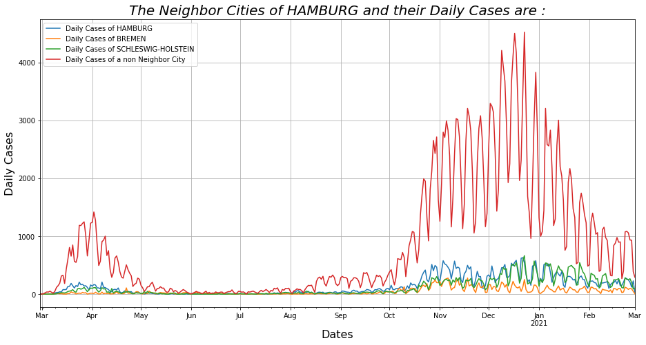
# This function finds neighbor cities of each city and plots their Daily Cases.
def find_neighbor_cities():
  # Import data from data.txt.
  cities_data = np.loadtxt("https://www.nickdoulos.com/assets/data.txt", delimiter=',', skiprows=1,
                          dtype = [('IDs','U3'), ('Cities', 'U30'), ('Dates', 'U25'), ('Cases', 'i4')])
  cities_name_df = pd.DataFrame(cities_data) # Make a dataframe of the cities data.
  # Drop the unused columns and duplicate values
  cities_name_df = cities_name_df.drop(columns =['IDs', 'Dates', 'Cases'], axis = 1).drop_duplicates()
  cities_df = pd.DataFrame(columns=['lat', 'lon', 'Neighbors'], index=range(15))
  cities_df.fillna(0.0)
  cities = cities_name_df['Cities'].values.tolist()
  geolocator = Nominatim(user_agent="geoapiExercises")
  cities_df['Cities'] = cities

  for idx, x in enumerate(cities_df['Cities']):
    location = geolocator.geocode(x).raw
    cities_df['lat'][idx] = location['lat']
    cities_df['lon'][idx] = location['lon']

  for i in range(15):
    neighbors = []
    for j in range(15):
      if i != j:
        if geodesic((cities_df['lat'][i], cities_df['lon'][i]),
                    (cities_df['lat'][j], cities_df['lon'][j])).km < 100:
            neighbors.append(cities_df['Cities'][j])
    cities_df['Neighbors'][i] = neighbors

  idCities =	{
    "BADEN-WURTTEMBERG": df1, "BAYERN": df2, "BRANDENBURG": df3, "BREMEN": df4, "HAMBURG": df5,
     "HESSEN": df6, "MECKLENBURG-VORPOMMERN": df7, "NIEDERSACHSEN": df8,
    "NORDRHEIN-WESTFALEN": df9, "RHEINLAND-PFALZ": df10, "SAARLAND": df11,
    "SACHSEN": df12, "SACHSEN-ANHALT": df13, "SCHLESWIG-HOLSTEIN": df14, "THURINGIA": df15
  }

  for i in range(15):
    if cities_df['Neighbors'][i] != []:
      variable_copy = idCities[cities_df['Cities'][i]]
      variable_copy.rename(columns = {'Daily Cases' : 'Daily Cases of ' + cities_df['Cities'][i]},
                           inplace = True)
      variable_copy = variable_copy.drop(['IDs', 'Cities', 'Cases'], axis=1)
      for j in cities_df['Neighbors'][i]:
        variable_copy = variable_copy.join(idCities[j], on='Dates', how='left')
        variable_copy = variable_copy.drop(['IDs', 'Cities', 'Cases'], axis=1)
        variable_copy.rename(columns = {'Daily Cases' : 'Daily Cases of ' + j}, inplace = True)
      for k in range(15):
        if cities_df['Neighbors'][k] == []:
          variable_copy = variable_copy.join(idCities[cities_df['Cities'][k]], on='Dates', how='left')
          variable_copy = variable_copy.drop(['IDs', 'Cities', 'Cases'], axis=1)
          variable_copy.rename(columns = {'Daily Cases' : 'Daily Cases of a non Neighbor City'},
                               inplace = True)
          break
      temp = variable_copy.reset_index().plot(x='Dates', figsize=(15.44, 7.70), grid=True)
      temp.set_title('The Neighbor Cities of ' + cities_df['Cities'][i]
                     + ' and their Daily Cases are :', fontsize=20, fontstyle='italic')
      temp.set_ylabel('Daily Cases', fontsize=16)
      temp.set_xlabel('Dates', fontsize=16)

find_neighbor_cities()
In the beginning of find_neighbor_cities() function, we set up the geolocator which is a library that with the help of which I look up the name of each city and store the Latitude and Longitude of each city and with the help of these values, we have the possibility to calculate the distance between the cities. If this distance is less than 100km then we consider one city as a neighbor of the other. We then create a dictionary with the names of the cities and the corresponding Data Frame to generate plots of the daily currencies of each set of neighboring cities together with a non-neighboring city to highlight the difference between neighboring and non-neighboring cities in the counts. The function displays all “sets” of cities but one of them for example is:
In the end, knowing the speed of Python, the program takes ~2.5 minutes to calculate the result, but only 30 seconds if you already know the 6 SARIMA variables and do not use the sarima_numbers_search() function.
You can also find the project on GitHub here.