Definition of Data Classification

Data classification is broadly defined as the process of organizing data by categories of information for data organizational purposes. Data classification is of particular significance when it comes to risk management, compliance, and data security.

Reasons for Data Classification

Data classification has improved significantly over time. Today, the technology is used for a variety of purposes, frequently in data security. Although, data may be classified for several reasons, including ease of access, maintaining regulatory compliance, and to meet various other business or particular goals.

Types of Learners in Classification

Lazy Learners

As the name suggests, similar kind of learners waits for the testing data to be appeared after storing the training data. Classification is done only after getting the testing data. They spend lower time on training but further time on prognosticating. Exemplifications of lazy learners are K-nearest neighbor and case-based reasoning.

Eager Learners

As contrary to lazy learners, eager learners construct classification model without waiting for the testing data to be appeared after storing the training data. They spend further time on training but lower time on prognosticating. Exemplifications of eager learners are Decision Trees, Naïve Bayes and Artificial Neural Networks (ANN).

Normalize or Standardize your Data?

Standardization: Standardization is a data processing workflow that converts the structure of different datasets into one common format of data. Variables that are measured at different scales might end up creating a bias.

Normalization: Likewise, the aim of normalization is to change the values of numeric columns in the dataset to a common scale, without distorting differences in the ranges of values. For machine learning, every dataset doesn’t bear normalization. It’s needed only when features have different ranges.

When should you use Normalization and Standardization

Normalization is useful when your data has varying scales and the algorithm you’re using doesn’t make hypotheticals about the distribution of your data, similar as k-nearest neighbors and artificial neural networks.

Example:

from sklearn.preprocessing import MinMaxScaler

scaler = MinMaxScaler()
data_scaled = scaler.fit_transform(data)

Standardization is useful when your data has varying scales and the algorithm you’re using does make hypotheticals about your data having a Gaussian distribution, similar as linear regression, logistic regression, and linear discriminant analysis.

Example:

from sklearn.preprocessing import StandardScaler

scaler = StandardScaler()
data_scaled = scaler.fit_transform(data)

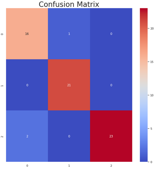
Classification Matrix

A classification matrix sorts all cases from the model into categories, by determining whether the prognosticated value matched the actual value. The classification matrix is a standard tool for evaluation of statistical models and is occasionally referred to as a confusion matrix.

Creating Train and Test assets

from sklearn.model_selection import train_test_split

train_set, test_set = train_test_split(data_frame, test_size = 0.3, random_state = 33, shuffle = True)

Were the parameter test_size = 0.3 suggests that the test data should be 30% of the dataset and the rest should be train data, the shuffle parameter that indicates whether the data should be shuffled before splitting, and when shuffle is True, random_state affects the ordering of the indices, which controls the randomness of each fold. Otherwise, this parameter has no effect.

Classification Algorithms

Logistic Regression

Logistic Regression is a statistical model used to determine which of the only two potential outcomes an independent variable has. It’s one among the only ML algorithms which will be used for various classification problems like spam spotting, Diabetes prediction, cancer detection etc. Logistic regression is simpler to implement, interpret, and effective to coach. However, Logistic Regression shouldn’t be used if the number of observations is lower than the number of features.

Naïve Bayes

Naïve Bayes algorithm is based on Bayes theorem and used for cracking classification problems. It’s not one algorithm but a family of algorithms. Naïve Bayes Classifier is one among the straightforward and best Classification algorithms which helps in assembling the fast machine learning models and will make quick forecasts. It’s used for a variety of tasks similar as spam filtering and other areas of text classification.

Naive Bayes algorithm is useful for:

• Naive Bayes is an easy and quick way to predict the class of the dataset.
• When the assumption of independence is valid, Naive Bayes is much more capable than the other algorithms like Logistic Regression.
• You require less training data.

Naive Bayes however, suffers from the following drawbacks:

• If the categorical variable belongs to a category that wasn’t followed up in the training set, then the model will give it a probability of 0.
• Naive Bayes assumes independence between its features.

Decision Tree

Decision Tree algorithms are used for both forecasts, as well as, classification in machine learning. The decision tree is a result of various hierarchical path that will help you to reach certain decisions. To assemble the tree, there are two steps – Induction and Pruning. In induction, we build a tree whereas, in pruning, we remove the several complexities of the tree.

K-Nearest Neighbors

K-nearest neighbors is one of the most basic, yet important classification algorithms in machine learning. KNNs have several operations in pattern recognition, data mining, and intrusion spotting. These KNNs are used in real- life scenarios where non-parametric algorithms are needed. These algorithms don’t make any hypotheticals about how the data is distributed. When we’re given previous data, the KNN classifies the coordinates into groups that are linked by a specific trait.

Support Vector Machine

Support Vector Machines algorithm provides analysis of data for classification and regression analysis. While they can be used for regression, SVM is substantially used for classification. We carry out plotting in the N-dimensional space (N = the number of features). The value of each point is also the value of the specified coordinate. To separate the two classes of data points, there are numerous possible hyperplanes that could be chosen. Our goal is to find a hyperplane that has the maximum distance between data points of both classes, so that future data points can be classified with further confidence.

How to know which Classification Algorithm to use

from sklearn.linear_model import LogisticRegression
from sklearn.neighbors import NearestNeighbors
from sklearn.neighbors import KNeighborsClassifier
from sklearn.tree import DecisionTreeClassifier
from sklearn.naive_bayes import GaussianNB
from sklearn.svm import SVC
from sklearn.model_selection import cross_val_score
from sklearn.model_selection import KFold
from sklearn.model_selection import GridSearchCV

models = []
models.append(('Logistic Regression', LogisticRegression()))
models.append(('K-Nearest Neighbors', KNeighborsClassifier()))
models.append(('Decision Tree', DecisionTreeClassifier()))
models.append(('Naive Bayes', GaussianNB()))
models.append(('Support Vector Machines', SVC()))

results = []
names = []
for name, model in models:
    kfold = KFold(n_splits = 2, random_state = 33, shuffle = True)
    cv_results = cross_val_score(model, X_train, y_train, cv = kfold, scoring = 'accuracy')
    results.append(cv_results)
    names.append(name)
    msg = "Scaled %s: %.2f%%" % (name, cv_results.mean()*100)
    print(msg)

In this block of code we evaluate the accuracy of each classification algorithm with the help of some functions. KFold (K-Folds cross-validator) provides train/test indices to split data in train/test sets. Split dataset into k consecutive folds. Each fold is then used once as a validation while the k - 1 remaining folds form the training set, were n_splits is the number of folds (must be at least 2). We also use cross_val_score to evaluate a score by cross-validation in which we use the model variable to pass all the algorithms we want to evaluate, then, the X_train is the data that we want to validate and the y_train the target of the X_train data. Also, the cv variable indicates the cross-validation splitting strategy, in this case K-Fold, and the scoring variable determinates the strategy to evaluate the performance data set. In the end we just print our resalts.

Example:
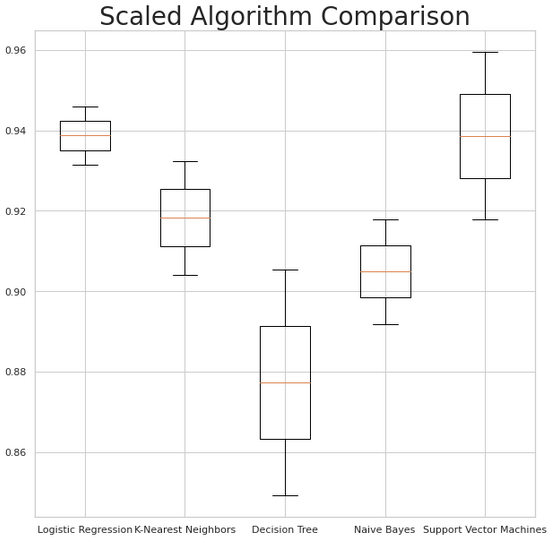
Scaled Logistic Regression: 93.87%
Scaled K-Nearest Neighbors: 91.83%
Scaled Decision Tree: 87.74%
Scaled Naive Bayes: 90.49%
Scaled Support Vector Machines: 93.86%

Plot the results to a Box Plot

import matplotlib.pyplot as plt
%matplotlib inline

fig = plt.figure()
ax = fig.add_subplot(111)
plt.boxplot(results)
ax.set_xticklabels(names)
fig.set_size_inches(10,10)
ax.set_title('Algorithm Comparison', size = 28)
plt.show()

In conclusion, here is an easy way to visually represent which of the classification algorithms have the better accuracy.

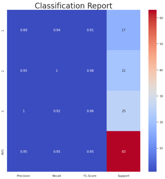
Bonus: A simple function that accepts the true test data and the predicted test data and creates a visual representation of a Classification Matrix and Report (Precision, Recall, F1-Score, Support).

from sklearn.metrics import confusion_matrix
from sklearn.metrics import precision_recall_fscore_support
import pandas as pd
import matplotlib.pyplot as plt
import numpy as np
import seaborn as sns
%matplotlib inline

def plot_classification_matrix_report(y_tru, y_prd, figsize=(11, 11), ax=None):

# Classification Matrix
  cm = confusion_matrix(y_tru, y_prd)
  plt.figure(figsize=(11,11))
  plt.title("Classification Matrix", size = 28)
  sns.heatmap(cm, annot=True, fmt='d', cmap="coolwarm");

# Classification Report (Precision, Recall, F1-Score, Support)
  plt.figure(figsize=figsize)
  plt.title("Classification Report", size = 28)
  xticks = ['Precision', 'Recall', 'F1-Score', 'Support']
  yticks = list(np.unique(y_tru))
  yticks += ['AVG']
  rep = np.array(precision_recall_fscore_support(y_tru, y_prd)).T
  avg = np.mean(rep, axis=0)
  avg[-1] = np.sum(rep[:, -1])
  rep = np.insert(rep, rep.shape[0], avg, axis=0)
  sns.heatmap(rep, annot=True, cbar=True, xticklabels=xticks, yticklabels=yticks, ax=ax, cmap="coolwarm")

plot_classification_matrix_report(test_true_data, test_predicted_data)